3.7. Inverse Distance Weighting
We can also interpolate a point layer to create a raster layer out of it. One method to do so is the Inverse Distance Weighting (IDW)
interpolation technique. To perform IDW interpolation in QGIS we have to rely on the external functionalities provided by GRASS GIS that
are directly accessible form the Processing Toolbox of QGIS.
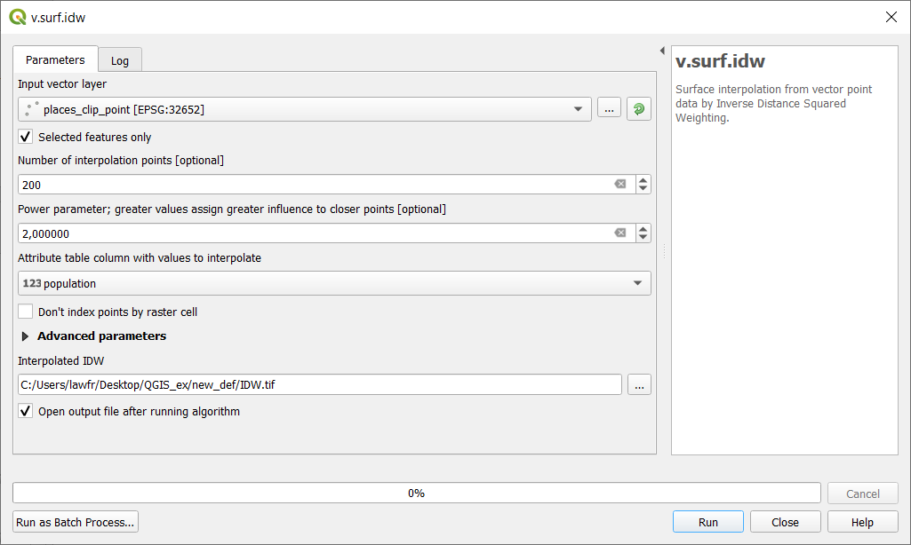
The function is called v.surf.idw, and it’s available at Processing Toolbox->GRASS->Vector(.v*). We can compute a raster by interpolating
the places_clip_point layer, using as the interpolation variable the population. But first, we need to select all the cities and towns that have a valid
population attribute (i.e. > 0): to do so, follow these steps:
- Right click on the
places_clip_pointlayer and open its Attribute table- Click on “Select features using an expression”
- In the window, write the following expression:
"population" > 0, and then click “Select features”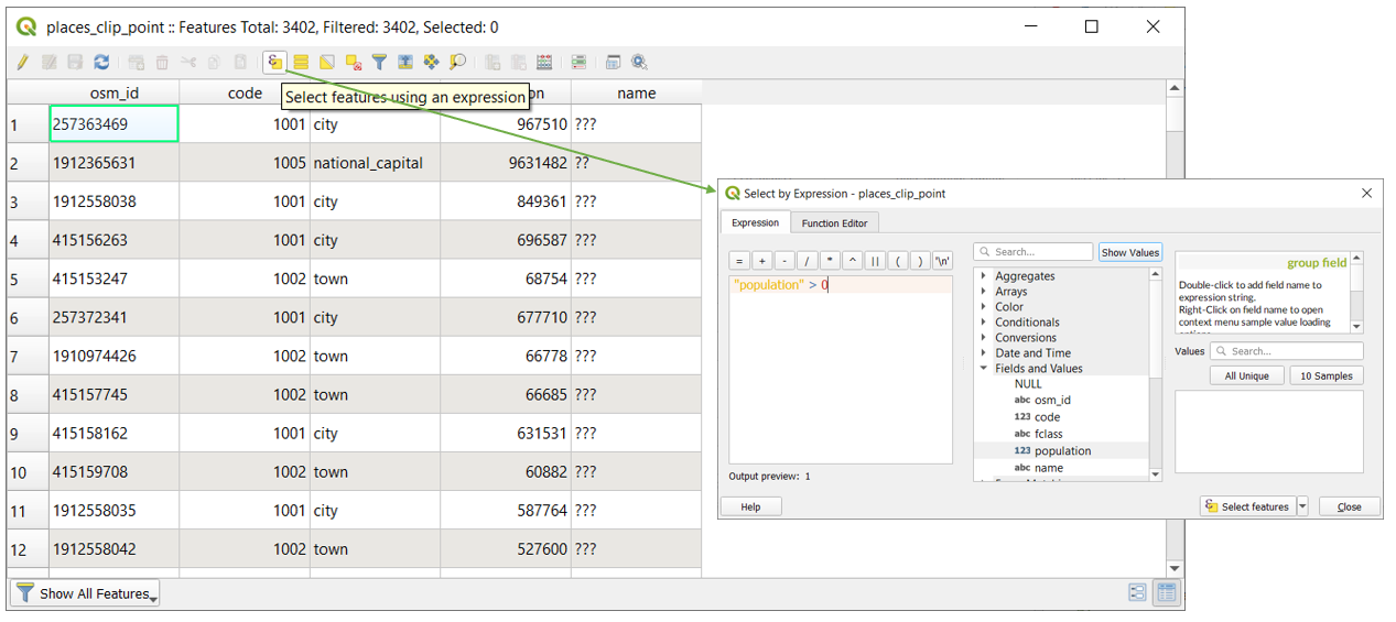
Now that we have selected all the places with population greater than 0, we can proceed with the IDW interpolation. Click on the v.surf.idw function and input the following parameters:
- Input vector layer: the
places_clip_pointlayer, be sure to tick the “Selected features only” option- Number of interpolation points: 200
- Attribute table column with values to interpolate: select “population”
- Interpolated IDW: the path and the name of the output raster layer. Note that if left empty a temporary layer will be created
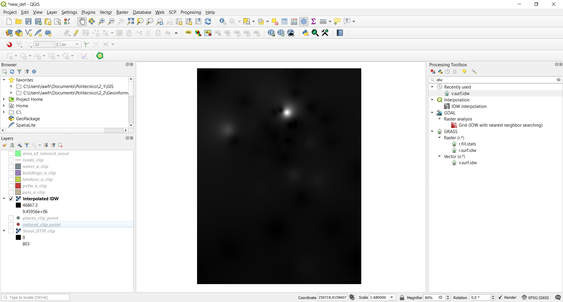
The result should initally look like this:
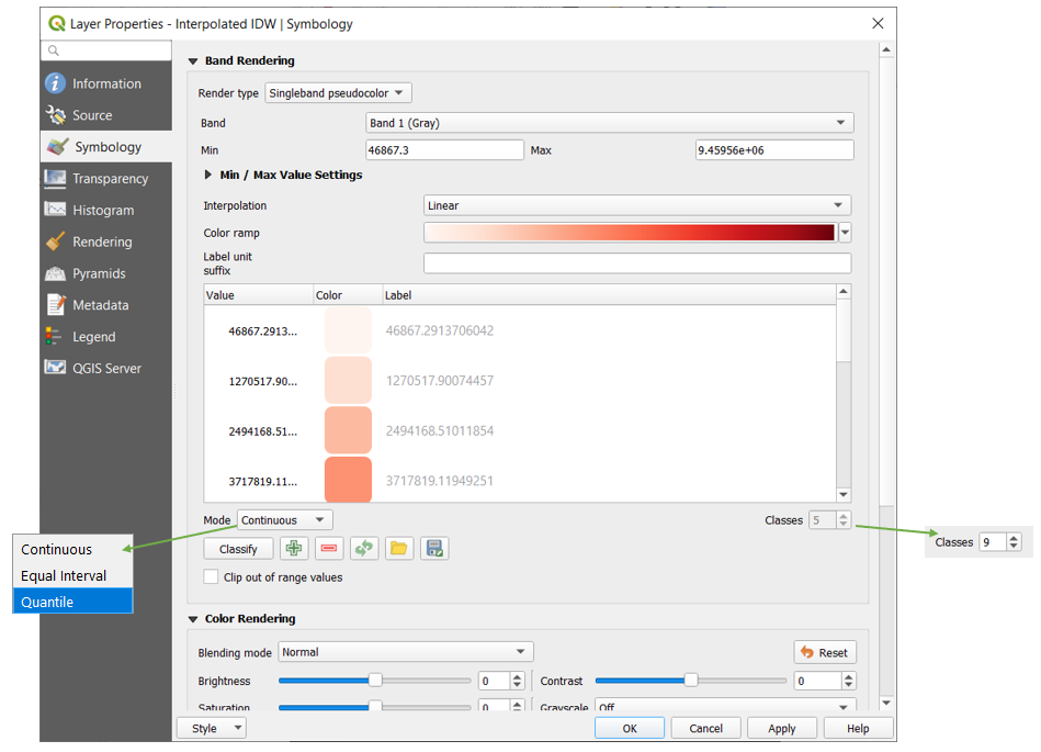
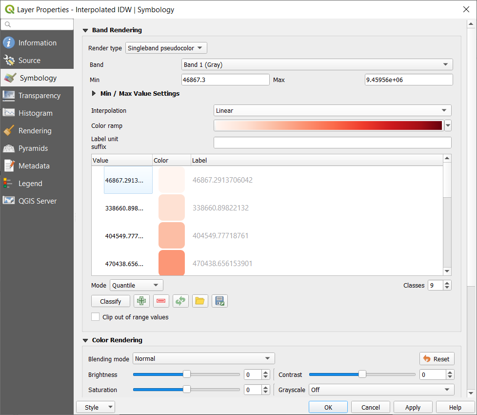
Since this result is not really optimal for an analysis, we can try to style it in a better way. To do so:
- Right-click on the newly created raster and click on “Properties”
- In the window, select “Symbology” from the menu on the left
- Change the first option (“Render type”) to “Singleband pseudocolor”
- Now change the classification mode to “Quantile”
- Change the number of classes to 9
- Click “Ok”
Now the result should be subdivided in 9 classes that contain an equal number of pixels each; the raster should look like this:
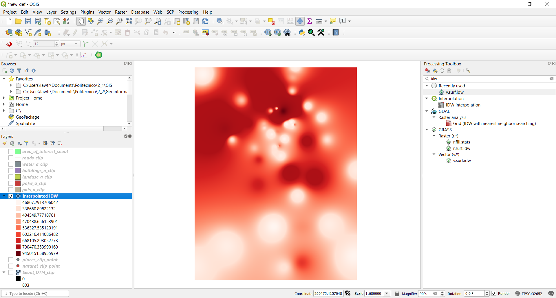
Fig. 3.7.1 Now it’s easier to distinguish the variation in population: note for example the dark red area in the top part of the image that represents the area where the capital Seoul is.